4.Data Reduction

4.1Load Calculation

The basic units utilized by geokon for measurement and reduction of data from vibrating wire load cells are digits. Calculation of digits is based on the following equation:

 

or

 

equation 1: Digits Calculation

To convert thef digits readings to load, the gauge readings for each cell must be averaged, and then the change in reading average multiplied by the gauge factor supplied with the load cell.

L = (R₁ – R₀) × G × K

equation 2: Load Calculation Using Linear Regression

Where:

L is the load in lb, kg, etc.

R₀ is the regression no-load reading in digits (average of all gauges).

R₁ is the current reading in digits (average of all gauges).

G is the gauge factor as supplied on the calibration sheet. As the load increases, the reading decreases, this gives G a negative sign when entered into the equation (see the example below).

K is the conversion factor (optional) as listed in the table below.

table 1: Engineering Units Conversion Multipliers

For example:

Model 4900 VW Load Cells have a regression no-load reading (R₀) of 7309 and a current average reading (R₁) of 5497, and the calibration factor is –397 lbs. per digit.

Inputting the values into Equation 2:

L = (5497 – 7309) × –397 = 719,400 lbs.

Note that the equations assume a linear relationship between load and gauge readings over the full load range, and the linear coefficient is obtained using regression techniques. Note that when using the calibration factor obtained from the regression formula it is necessary to use the regression zero. This may introduce substantial errors at very low loads. A measure of the amount of nonlinearity is shown on the calibration sheet in the column entitled Linearity. See Appendix F for additional information.

For greater accuracy, the data given can be represented by a polynomial or can be treated as a series of segments over the entire load range. For instance, using the example calibration sheet, the load between 0 and 180,000 lb could be represented by the equation:

L = ((7304 – 6860) × 405 = 179,820 tons.

The gauge factor –405 lb/digit is calculated from the slope of the line between a load of 0 and 180,000 lb, i.e., (0 – 180,000) / (7304 – 6860) = –405 lb/digit.

A polynomial expression to fit the data is shown in Equation 3.

L = AR₁² + BR₁ + C

equation 3: Load Calculation Using Polynomial

Where:

L is the load in lb, kg, etc.

R₁ is the current reading (average of all gauges).

A, B, and C are the coefficients derived from the calibration data.

First calculate C from the initial average field zero reading.

For example: if C = 7,305 then 0 = –0.00247 × 73,052 – 367 × 7,305 + C from which C = +2,812,740. Therefore, when the applied load is 360,000, R₁ = 6,409, and the calculated load = –0.00247 × 64,092 – 367 × 6,409 + 2,812,740 = 359,180 lbs.

4.2Temperature Correction Factor

A small correction can be made for change in temperature. As the temperature goes up the average reading of all the sensors will go down approximately one digit per °C. To calculate the load, corrected for temperature, use Equation 4.

L = G [(R₁ – R₀) + (T₁ – T₀)]

equation 4: Load, Corrected for Temperature

The temperature effect shown above is for a load cell that has not been installed yet and is very minor. There is no telling what the actual temperature effect will be on a load cell that is installed on a tensioned bar or cable. This depends on the length of the bar or cable and on the properties of the surrounding ground. The actual temperature effect can only be arrived at empirically by simultaneous measurements of load and temperature over a short period of time.

 

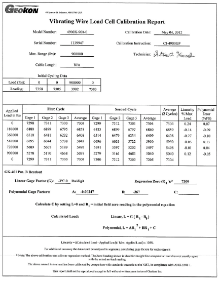
Figure 9: Typical Model 4900 Calibration Sheet